
Microsoft Excel provides a great feature, Conditional Formatting, to apply the formatting to particular Cells when the given criteria are met. We can apply the formatting to a particular cell or range of cells. You need to select the Rule depending on your requirements to colorize or format the cells.
In this article, I am going to explain how to apply Conditional Formatting for the selected Cells in Microsoft Excel 2013. The steps may be the same for other versions of Excel.
How to Apply Conditional Formatting?
Step 1. Open the Excel file where you have the data and would like to use Conditional Formatting.
Step 2. Select the Cells to apply the color based on a certain condition.
Step 3. Select the HOME tab. Then select the “Conditional Formatting” icon from the “Styles” group. Microsoft Excel displays a menu and then selects the “New Rule…” menu item.

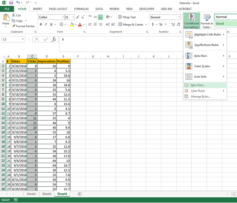
Excel opens the “New Formatting Rule” dialog to allow you to select the rule; for the selected cells to apply the format.
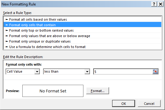
Step 4. From the “New Formatting Rule” dialog, you need to select the right Rule Type from “Select a Rule Type:” depending on your requirement.

Step 5. You can select the below Rule Types:
- Format all cells based on their values
- Format only cells that contain particular values
- Format only top or bottom-ranked values
- Format only values that are above or below average
- Format only unique or duplicate values AND
- Use a formula to determine which cells to format
For example, I want to apply the color to the selected Cells; if the cell value is < 5. To do this; select the relevant Rule Type, which is “Format only cells that contain” from the “Select a Rule Type:” list.
Step 6. Once you select the Rule Type; Excel will display relevant fields to set the condition under the “Edit the Rule Description:” field.
Our requirement is to format the cells; based on their value. So, select the below values from the “Format only cells with:” fields:
- Cell Value” and then select “less than” and then give the value 5. That means, format only cells with a Cell Value less than 5.
Step 7. Then we need to apply the format. Click on the “Format…” button. Excel opens the “Format Cells” dialog. I want to fill the cells with RED color.
So, select the “Fill” tab and then select the RED color. You will see the full-color preview in the “Sample” section.
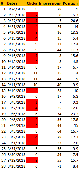
Step 8. Click on the OK button to set the Color. And then click on the OK button from the “New Formatting Rule” dialog to Apply the color to the selected cells based on the selected rule. Once the conditional formatting is applied, the selected Cells are colorized and look like the below:

We discuss more Excel through my Articles.
Please give your feedback through the below Comments.
🙂 Sahida